Backtesting Mad-Money recommendations and the Cramer-effect
Can we profit from the recommendations of the stock picking guru?
- 11 minsWhen it comes to trading, investors are listening a lot on other people opinions without looking into the data and the background of the company. And the more credible (at least in theory) the source is, the more people pay attention without any second thought. This is the case with the show Mad Money on CNBC [1] with the host Jim Cramer. In this post I will show you how the “Mad Money” portfolio could have performed and what the Cramer-effect [4] looks like (if there is such a thing).
To achieve this, I scraped the historical buy recommendations from the show, then backtested every company which was on the list as a “buy recommendation”.
Find the GitHub repo with all the code and data used to write this post: https://github.com/gaborvecsei/Mad-Money-Backtesting

The Cramer-effect and his recommendations
The Cramer-Effect (Cramer Bounce):
After the show Mad Money the recommended stocks are bought by viewers almost immediately (after hours trading) or on the next day at market open, increasing the price for a short period of time. [4]
This is really interesting but not surprising as I already pointed out in the intro how this works for most people. Kind of sad, but who doesn’t want to get rich without any work 🤑?
Other that this I wanted to take a bigger timeframe and see what would have happened if I follow the investment ideas of the stock picking guru and his team.
Recommendations data from the show
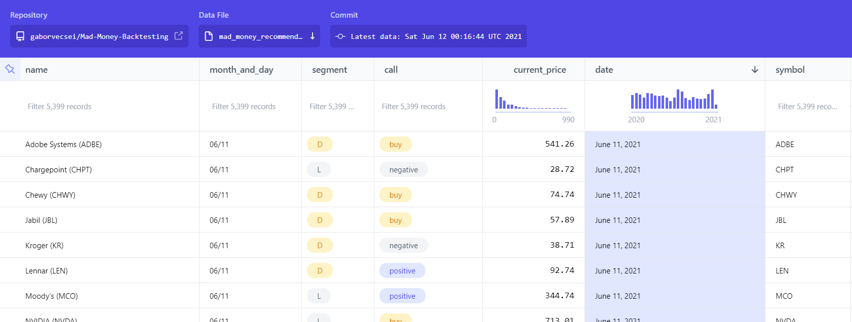
Fortunately the data is available, as Cramer’s team makes it available via their own website [2], we just need to get it from there.
You can find a table on the site which holds the mentioned stocks and actions on the show for a single day. As you can see there are some basic options where we can select a price threshold, and most importantly the day, when there was a show. If we look closely and investigate the HTTP request (via the browsers dev mode), we can see that a simple POST request is sent with some form data (application/x-www-form-urlencoded) which contains the different “filterings”. This can be easily constructed, so once we have the contents of the page, we only need to parse it. I used BeautifulSoup for that.
You can try this for yourself with this little script.
Automation w/ GitHub Actions
Let’s be honest, we can do much better than manually preparing the data. Even better, as the resulting file is not huge, we can keep it in the version control system. This is not just a fancy addition, but can actually help as it can be directly used by everyone and more importantly, we can see the change in the contents of the file over time. Maybe you think it’s not a big deal, but this way, if there would be a “problem” on the Mad Money crew’s end, and they would mess up recommendations for some dates (in the present everyone is smarter about the past 😉, wink wink) then we would see it. We can get rid of the “it’s working on my computer” but for data problem.
Also, with the Flat Data Viewer [3], we get a cool visualization: https://flatgithub.com/gaborvecsei/Mad-Money-Backtesting
This is all achieved with GitHub Actions. Without going into the details it’s as simple as:
- Checkout master branch
- Prepare Python with the necessary dependencies
- Use the scraper code to retrieve and transform the data
- If there was a change in the contents of the
.csvfile, then let’s commit it - Enjoy the fruits of this really cool feature
(Idea is from [7])
Backtesting
As everything is covered: what is the goal, how we got the data, we can start to look into the backtesting and the results.
For the backtesting I used the backtesting.py [5] package (The backtrader is just as good) and yfinance [6] with which I got the historical stock data.
For the simulations, each mentioned stock is tested individually, then the overall results are calculated. (We also store the individual results in a html file.) I prepared a predefined amount which I would invest in a stock. This stays the same no matter the company, as we want to spend equally as we don’t know how the stock will perform. At each buy recommendation we go “all in” and buy as many positions as we can with the money. Once we sell, then we sell all of it. The buy and sell dates are defined in the backtesting classes, and they are “calculated” from the recommendation dates.
$\text{Recommendation dates} \rightarrow \text{Buy dates} \rightarrow \text{Sell dates}$
If a company was mentioned more times, then based on the strategy we can buy and sell more times.
Challenges
Before I show the results, I would like to write a bit about the challenges. These are important factors as all of them can alter the results at the end.
Fortunately if you have better data, then it is easily curable.
After hours data
This is one of the biggest problems 😢 as we literally don’t have it. It’s a bit of an over exaggeration, as yfinance can provide it but it is sparse. I solved this by stating that the price at showtime is the same as it is at market close. Of course with this (dummy) extrapolation, we cannot count on the profits/losses of the after-hours volatility which would be generated (in theory) by the show.
If you have (maybe a paid) data resource, then by adjusting the buy/sell date calculations, you can easily adapt the strategies to a proper after-hours trading session which would provide the accurate results for the Cramer effect.
Missing days
There are a few days for each stock, where we have missing data. The problem comes in when we had a recommendation around that date and we would like to buy/sell on the missing day. To overcome this problem I made a simple function with which you can transform these dates at buy/sell date calculation. Either you drop it, or use the next “closest” date.
Dropping would mean, that we won’t buy/sell on the date at all, while using the closest date could result in lower accuracy in returns, as that is also an approximation. Btw. if in the real-life scenario we would not strictly follow the buy patterns, and would buy max few business day later, than that would match with this approximation.
Data Quality
I don’t have any measures for this, but as I saw free sources of financial data have their own problems and they are usually not accurate. When measuring short term effects, few cents can make a difference. We need to keep this in our minds as well.
(But take this point with a grain of salt, as I only used free data sources.)
Trading Strategies
Multiple trading strategies are implemented to test the Cramer effect and his “portfolio”:
- $A$) BuyAndHold (and repeat)
- The stocks are bought at the first mention on the show, then held for $N$ days. On the $N$th day the positions are closed. If there were other mentions after we sold, we repeat this process. (If at the end of the simulation we still have open positions, those are closed automatically)
- $B$) AfterShowBuyNextDayCloseSell
- We buy the mentioned stocks at the end of the show and then sell on the next day at market Close
- $C$) AfterShowBuyNextDayOpenSell
- We buy the mentioned stocks at the end of the show and then sell on the next day at market Open
- $D$) NextDayOpenBuyNextDayCloseSell
- We buy the mentioned stocks at next day market open and then sell it on the same day at market close
The Cramer-effect is simulated with strategies $B$, $C$ and $D$, as we are aiming for the short-term effect. Strategy $D$ is the one, where no after-hours trading is involved.
Results
Results are obtained by observing stock values and company mentions from 2020-01-01 to 2021-06-04.
At every show there are “buy” recommendations and also “positive” mentions. The latter means that there is a bigger chance to see bullish market, but it’s not as strong signal as the buy recommendation. In conclusion we should see more consistent returns with the buy signals. This is what I used for the backtesting.
For each unique stock I invested \$1000 and set a commission of 2%
(In the code there is an option to use stop-loss and take-profit, but results were calculated without these).
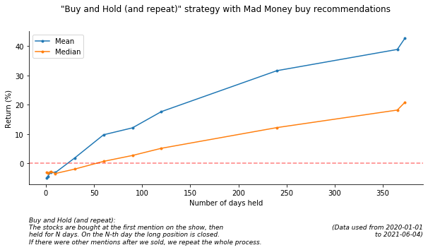
Buy and Hold (and repeat)
| Days Held | Negative Returns | Positive Returns | Mean Return % | Median Return % |
|---|---|---|---|---|
| 1 | 543 | 170 | -4.85436 | -3.01154 |
| 2 | 523 | 190 | -4.38844 | -3.3714 |
| 5 | 481 | 232 | -3.03959 | -2.72434 |
| 10 | 455 | 258 | -3.09772 | -3.42916 |
| 30 | 385 | 328 | 1.84899 | -1.93449 |
| 60 | 348 | 365 | 9.75003 | 0.699654 |
| 90 | 329 | 383 | 12.1096 | 2.70547 |
| 120 | 295 | 418 | 17.6343 | 5.15033 |
| 240 | 227 | 486 | 31.5762 | 12.1968 |
| 365 | 215 | 498 | 38.8041 | 18.1675 |
| 373 | 185 | 528 | 42.6746 | 20.8505 |
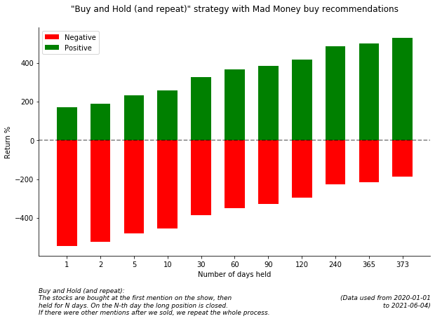
(at this last plot the y axis is count and not Return)
Cramer Effect
These are the short term trading strategies which I tested.
| Strategy | Negative Returns | Positive Returns | Mean Return % | Median Return % |
|---|---|---|---|---|
| AfterShowBuyNextDayCloseSell | 546 | 166 | -5.01226 | -3.12014 |
| AfterShowBuyNextDayOpenSell | 570 | 142 | -5.10033 | -3.16921 |
| NextDayOpenBuyNextDayCloseSell | 543 | 169 | 0.83846 | -2.9403 |
In the repo, under the art/ folder you should find visualizations for the results of each strategy.
Conclusion
From the Buy and Hold results it is visible that creating a diverse portfolio and holding the positions results in greater returns. So no magic 🧙 here, just the golden rule of investing - be diverse and hold 💎👐. (Also don’t forget that the tested period was bullish most of the time, so it was “easier” to generate profits).
Of course this is nowhere near a real-life scenario. Let’s think about it: there are more than 700 unique stocks and I invested \$1000 per stock. At the end this resulted in a more than \$700,000 investment. We could fix this buy using a smaller amount, which would exclude stocks to buy then, or we could set an amount per day and based on some logic select positions to buy, which again, results in excluding stocks.
On the Cramer-Effect and short-term investment results, I don’t have any convincing results. Based on these numbers I would say that the Cramer effect is not present, but keep in mind that I used multiple approximations because of the incomplete/missing data. So if there would be a small upside, then we would not catch it this was. But it is true that there are no short term significant returns based on these strategies.
References
[1] Mad Money show
[7] Git scraping: track changes over time by scraping to a Git repository

Gábor Vecsei
I love chocolate